Case Study - Effects of snow cover characteristics and reproduction on body mass in bighorn sheep (Ovis canadensis)

Here, we display the use of the visualization method for indirect effects with a real-world example of the carry-over effects of snow cover characteristics on subsequent spring and automn mass of bighorn sheep on Ram mountain (Alberta, CAN). The original article by Crémel et al. can be found at LINK. This use case is more complex than the ones presented in the original article describing the method (LINK) as there is more than one mediator involved and in some cases, the exposure interacts with a mediator and in another case, the exposure interacts with a mediator and both mediators interact with one-another. We will display how the visualization method can be used to make such complex relationships more intuitive to interpret.

The full DAGs for the three analyses we will be working here can be found below:

To better understand the DAGs and relationships, readers are referred to the original publication.

Set up workspace

Load packages

library(tidyverse)
library(brms)
library(cmdstanr)
library(tidybayes)
library(ggpubr)
library(marginaleffects)
library(splines)
library(patchwork)

Load data and models

data_all <- readRDS("mass_loss_data_all_Kallan_Cremel.rds")

# Female data and model
## data
Data_females_uns <- data_all$Data_females_uns 

## Model
Mass_loss_female_repro_int <- readRDS("Mass_loss_female_repro_int_uns_Kallan_Cremel.rds")

# Lamb data and model
## data
Data_lambs_uns <- data_all$Data_lambs_uns


## Model
Mass_loss_lamb <- readRDS("Mass_loss_lamb_uns_Kallan_Cremel.rds")

# Male data and model
## data
### Scaled (for model)
Data_male_scaled <- data_all$Data_male_scaled
### Unscaled (for unscaling predictions)
Data_males_uns <- data_all$Data_males_uns

## Model
Mass_loss_male_pop <- readRDS("Mass_loss_male_pop_Kallan_Cremel.rds")

Female model

Here, we look at the following DAG: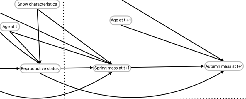

We will focus on Snow characteristics, reproductive status, spring mass t+1, and autumn mass t+1. In the model, snow characteristics is actually three variables that each interact with Reproductive status for their respective effects on spring mass t+1. Then, Spring mass t+1 interacts with reproductive status for its effect on autumn mass t+1.

The three-equation model is defined in brms as such:

f_repro <- bf(lead_repro ~ 1 + ns(Age, 3) + wtd114 + pop_den + avg_snow_depth + days_count + median_density + (1 | ID) + (1 | Yr), 
              family = bernoulli(link = "logit"))

f_t_int <- bf(next_wtd12 ~ 1 + wtd114 + ns(Age, 3) + pop_den + 
              lead_repro * avg_snow_depth + 
              lead_repro * days_count + 
              lead_repro * median_density + 
              (1 | ID) + (1 | Yr), 
              family = gaussian())

f_t1 <- bf(wtd114_next ~ 1 + lead_repro*next_wtd12 + ns(Age_next, 3) + pop_den_next + (1 | ID) + (1 | Yr_next), 
           family = gaussian())

Mass_loss_female_repro_int <- brm(
  f_repro + f_t_int + f_t1,
  data = Data_females_uns, 
  set_rescor(FALSE), 
  cores = 4, threads = threading(2), backend = "cmdstanr",warmup = 2000, iter = 6000, chains = 4
)

Crémel et al. plot all of the direct effects in the DAG so we will not be repeating this here. We will only focus on the interacting effect of snow variables with reproductive status on spring mass and the interacting effect of spring mass and reproductive status on autumn mass. For the demonstration, we will work only with Average snow depth as the Snow variable. See Crémel et al. for all indirect effects.

Spring mass ~ Snow * Reproductive status

col_repro <- c("Non-reproductive" = "#d95f02", "Reproductive" = "#2ca25f")

p_smass_snow <- predictions(Mass_loss_female_repro_int,
                           newdata = datagrid(avg_snow_depth = seq(from = min(Data_females_uns$avg_snow_depth),
                                                                    to = max(Data_females_uns$avg_snow_depth),
                                                                    by = 1),
                                               lead_repro = c(0,1)),
                           re_formula = NA,       # Population-level predictions
                           type = "response",     # epred
                           resp = "nextwtd12") |> # spring mass
               get_draws(shape = "rvar") |>       # convert to rvar
               mutate(Reproduction_status = factor(lead_repro, 
                                      levels = c(0, 1), 
                                      labels = c("Non-reproductive", "Reproductive"))) 

Loading required namespace: rstan

plot_smass_snow <- ggplot() +
  stat_lineribbon(data = p_smass_snow, aes(x = avg_snow_depth, ydist = rvar, fill = Reproduction_status),
                  .width = seq(0.5, 0.95, length.out = 20), 
                  alpha = 0.05, color = "black") +
  guides(fill = guide_legend(override.aes = list(alpha = 1, fill = NA, color = col_repro))) +
  scale_fill_manual(values = col_repro) +
  labs(
    x = "Average snow depth (cm)",
    y = "Spring mass (kg)",
    fill = "Reproduction status (t+1)"
  ) +
  theme_pubr() +
  theme(legend.position = "inside",
        legend.position.inside = c(0.2, 0.2))

plot_smass_snow

Autumn mass ~ Spring mass * Reproductive status

p_amass_smass <- predictions(Mass_loss_female_repro_int,
                           newdata = datagrid(next_wtd12 = seq(from = min(Data_females_uns$next_wtd12),
                                                                    to = max(Data_females_uns$next_wtd12),
                                                                    by = 1),
                                               lead_repro = c(0,1)),
                           re_formula = NA,         # Population-level predictions
                           type = "response",       # epred
                           resp = "wtd114next") |>  # autumn mass
               get_draws(shape = "rvar") |>         # convert to rvar
               mutate(Reproduction_status = factor(lead_repro, 
                                      levels = c(0, 1), 
                                      labels = c("Non-reproductive", "Reproductive"))) 

plot_amass_smass <- ggplot() +
  stat_lineribbon(data = p_amass_smass, aes(x = next_wtd12, ydist = rvar, fill = Reproduction_status),
                  .width = seq(0.5, 0.95, length.out = 20), 
                  alpha = 0.05, color = "black") +
  scale_fill_manual(values = col_repro) +
  guides(fill = guide_legend(override.aes = list(alpha = 1, fill = NA, color = col_repro))) +
  labs(
    x = "Spring mass (kg)",
    y = "Autumn mass (kg)",
    fill = "Reproduction status (t+1)"
  ) +
  theme_pubr() +
  theme(legend.position = "inside",
        legend.position.inside = c(0.2, 0.8))

plot_amass_smass

Indirect effect of snow on autumn mass

Predictions

We want to predict autumn mass from the predicted values of spring mass as a function of snow depth and reproductive status

# the estimate column of p_smass_snow is the median of the posterior distribution
# Let's simplify the prediction object to work with after
p_smass_snow |> 
  as_tibble() |> 
  select(estimate, avg_snow_depth, lead_repro) |>
  rename(next_wtd12 = estimate) -> spring_mass_pred

# Custom prediction grid
datagrid(model = Mass_loss_female_repro_int,
         next_wtd12 = spring_mass_pred$next_wtd12) |>
  # need to add lead_repro separately as grid_type = "dataframe" argument throws an error
  select(-lead_repro) |>      
  left_join(spring_mass_pred |> select(next_wtd12, lead_repro)) -> f_snow_indirect_pred_grid

# Predictions
p_ind_snow_smass <- predictions(Mass_loss_female_repro_int,
                           newdata = f_snow_indirect_pred_grid,
                           re_formula = NA,         # Population-level predictions
                           type = "response",       # epred
                           resp = "wtd114next") |>  # autumn mass
                    mutate(Reproduction_status = factor(lead_repro, 
                                      levels = c(0, 1), 
                                      labels = c("Non-reproductive", "Reproductive"))) |>
              # Add snow values from spring mass prediction grid
                    select(-avg_snow_depth) |>
                    left_join(spring_mass_pred)

plot

COLS <- alpha(colorRampPalette(c("#f7fcf9","#0b6da7b7"))(30),0.8)

plot_amass_smass + 
  geom_line(data = p_ind_snow_smass, aes(x = next_wtd12, y = estimate, color = avg_snow_depth, linewidth = avg_snow_depth, group = Reproduction_status), lineend = "round") +
  scale_color_gradientn(colours = COLS, name = "Avg Snow Depth") +
  guides(linewidth = "none") +
  theme(legend.direction = "horizontal",
        legend.position = "bottom")

The indirect effect is small compared to the direct effect so let’s zoom in a little

plot_amass_smass + 
  geom_line(data = p_ind_snow_smass, aes(x = next_wtd12, y = estimate, color = avg_snow_depth, linewidth = avg_snow_depth, group = Reproduction_status), lineend = "round") +
  scale_color_gradientn(colours = COLS, name = "Avg Snow Depth") +
  guides(linewidth = "none") +
  theme(legend.direction = "horizontal",
        legend.position = "bottom") +
  coord_cartesian(xlim = c(50, 60), ylim = c(60, 80))

Lamb model

Here, we look at the following DAG:

We will focus on Snow characteristics, sex, spring mass t+1, and autumn mass t+1. In the model, snow characteristics is actually three variables that each interact with sex for their respective effects on spring mass t+1. Then, Spring mass t+1 interacts with sex for its effect on autumn mass t+1.

The two-equation model is defined in brms as such:

f_lamb_t <- bf(next_wtd12 ~ 1 + Sex*(wtd114  + pop_den + avg_snow_depth + days_count + median_density) + (1 | Yr), family = gaussian())

f_lamb_t1 <- bf(wtd114_next ~ 1 + Sex*(next_wtd12 + pop_den_next) + (1 | Yr_next), family = gaussian())
 
Mass_loss_lamb <- brm(
  f_lamb_t + f_lamb_t1,
  data = Data_lambs_uns, set_rescor(FALSE), cores=4, threads = threading(2), backend="cmdstanr", warmup = 2000, iter = 6000
) 

Crémel et al. plot all of the direct effects in the DAG so we will not be repeating this here. We will only focus on the interacting effect of snow variables with sex on spring mass and the interacting effect of spring mass and sex on autumn mass. For the demonstration, we will work only with Average snow depth as the Snow variable. See Crémel et al. for all indirect effects.

Spring mass ~ Snow * Reproductive status

col_sex <- c("Male" = "#d95f02", "Female" = "#2ca25f")

p_smass_snow_lambs <- predictions(Mass_loss_lamb,
                           newdata = datagrid(avg_snow_depth = seq(from = min(Data_lambs_uns$avg_snow_depth),
                                                                    to = max(Data_lambs_uns$avg_snow_depth),
                                                                    by = 1),
                                               Sex = c("Male", "Female")),
                           re_formula = NA,       # Population-level predictions
                           type = "response",     # epred
                           resp = "nextwtd12") |> # spring mass
               get_draws(shape = "rvar")          # convert to rvar

plot_smass_snow_lambs <- ggplot() +
  stat_lineribbon(data = p_smass_snow_lambs, aes(x = avg_snow_depth, ydist = rvar, fill = Sex),
                  .width = seq(0.5, 0.95, length.out = 20), 
                  alpha = 0.05, color = "black") +
  guides(fill = guide_legend(override.aes = list(alpha = 1, fill = NA, color = col_sex))) +
  scale_fill_manual(values = col_sex, labels = c("Male", "Female")) +
  labs(
    x = "Average snow depth (cm)",
    y = "Spring mass (kg)",
    fill = "Sex"
  ) +
  theme_pubr() +
  theme(legend.position = "inside",
        legend.position.inside = c(0.2, 0.2))

plot_smass_snow_lambs

Autumn mass ~ Spring mass * Sex

p_amass_smass_lambs <- predictions(Mass_loss_lamb,
                           newdata = datagrid(next_wtd12 = seq(from = min(Data_lambs_uns$next_wtd12),
                                                                    to = max(Data_lambs_uns$next_wtd12),
                                                                    by = 1),
                                               Sex = c("Male", "Female")),
                           re_formula = NA,         # Population-level predictions
                           type = "response",       # epred
                           resp = "wtd114next") |>  # autumn mass
               get_draws(shape = "rvar")            # convert to rvar

plot_amass_smass_lambs <- ggplot() +
  stat_lineribbon(data = p_amass_smass_lambs, aes(x = next_wtd12, ydist = rvar, fill = Sex),
                  .width = seq(0.5, 0.95, length.out = 20), 
                  alpha = 0.05, color = "black") +
  scale_fill_manual(values = col_sex, labels = c("Male", "Female")) +
  guides(fill = guide_legend(override.aes = list(alpha = 1, fill = NA, color = col_sex))) +
  labs(
    x = "Spring mass (kg)",
    y = "Autumn mass (kg)",
    fill = "Sex"
  ) +
  theme_pubr() +
  theme(legend.position = "inside",
        legend.position.inside = c(0.2, 0.8))

plot_amass_smass_lambs

Indirect effect of snow on autumn mass

Predictions

We want to predict autumn mass from the predicted values of spring mass as a function of snow depth and Sex

# the estimate column of p_smass_snow is the median of the posterior distribution
# Let's simplify the prediction object to work with after
p_smass_snow_lambs |> 
  as_tibble() |> 
  select(estimate, avg_snow_depth, Sex) |>
  rename(next_wtd12 = estimate) -> spring_mass_pred_lambs

# Custom prediction grid
datagrid(model = Mass_loss_lamb,
         next_wtd12 = spring_mass_pred_lambs$next_wtd12) |>
  # need to add Sex separately as grid_type = "dataframe" argument throws an errorr
  select(-Sex) |>      
  left_join(spring_mass_pred_lambs |> select(next_wtd12, Sex)) -> f_snow_indirect_pred_grid_lambs

# Predictions
p_ind_snow_smass_lambs <- predictions(Mass_loss_lamb,
                           newdata = f_snow_indirect_pred_grid_lambs,
                           re_formula = NA,         # Population-level predictions
                           type = "response",       # epred
                           resp = "wtd114next") |>  # autumn mass
              # Add snow values from spring mass prediction grid
                    select(-avg_snow_depth) |>
                    left_join(spring_mass_pred_lambs)

plot

COLS <- alpha(colorRampPalette(c("#d0ddd6","#47a6ddb7"))(30),0.8)

plot_amass_smass_lambs + 
  geom_line(data = p_ind_snow_smass_lambs, aes(x = next_wtd12, y = estimate, color = avg_snow_depth, linewidth = avg_snow_depth, group = Sex), lineend = "round") +
  scale_color_gradientn(colours = COLS, name = "Avg Snow Depth") +
  guides(linewidth = "none") +
  theme(legend.direction = "horizontal",
        legend.position = "bottom")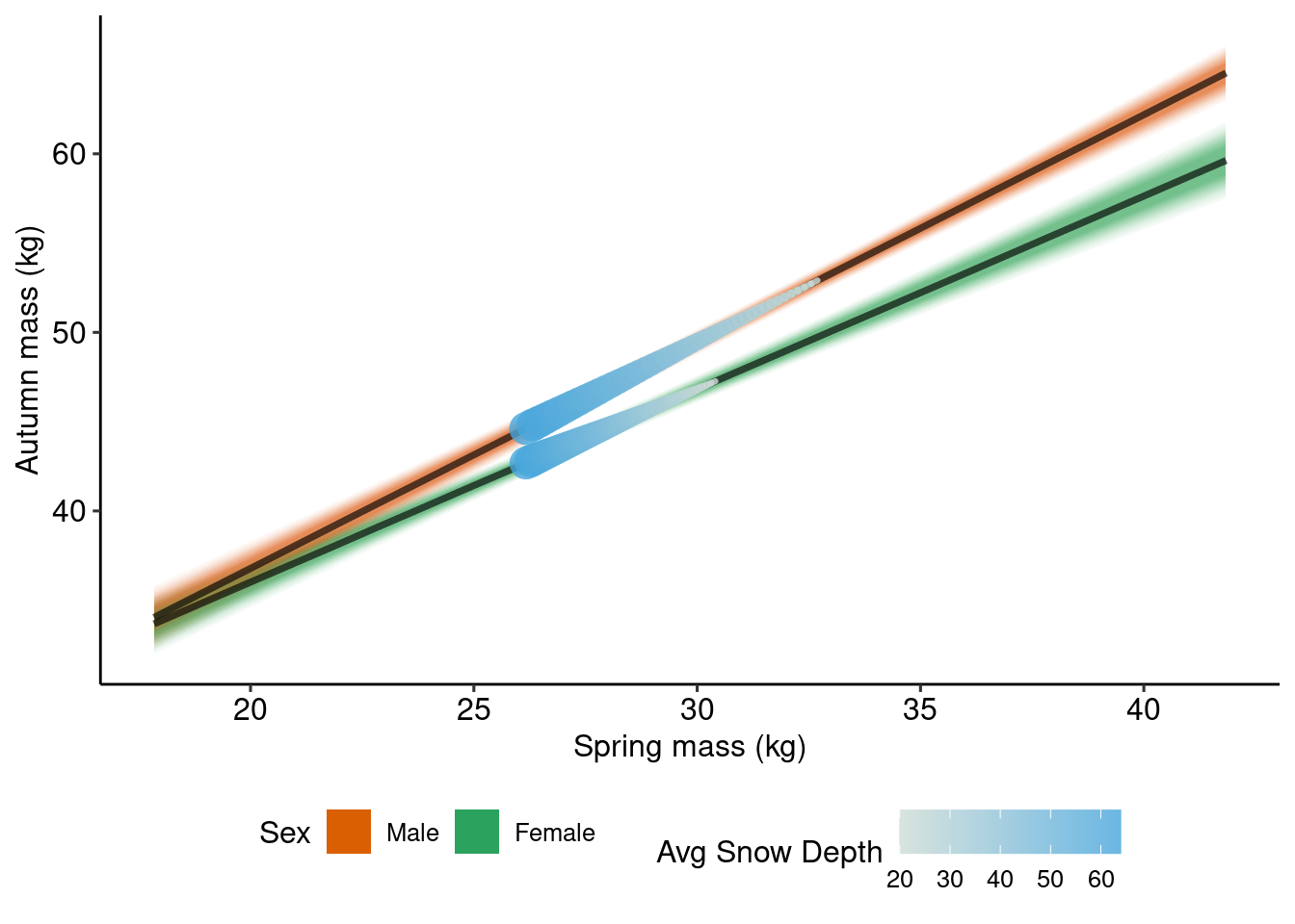

Male model

Here, we look at the following DAG:

We will focus on Snow characteristics, sex, spring mass t+1, and autumn mass t+1. In the model, snow characteristics is actually three variables that each interact with population density for their respective effects on spring mass t+1. However, in this case, Spring mass t+1 dopes not interact with population density for its effect on autumn mass t+1. There still will be an interaction present in the indirect effects but not through the mediator most immediate to the outcome.

The two-equation model is defined in brms as such:

f_male_t1 <- bf(wtd114_next ~ 1 + scale(next_wtd12) + ns(Age_next, 3) + pop_den_next + (1 | ID) + (1 | Yr_next), family = gaussian())

f_male_pop_t <- bf(next_wtd12 ~ 1 + wtd114 + ns(Age, 3) + 
                   pop_den * avg_snow_depth + 
                   pop_den * days_count + 
                   pop_den * median_density + 
                   (1 | ID) + (1 | Yr), 
                   family = gaussian())

Mass_loss_male_pop <- brm(
  f_male_pop_t + f_male_t1,
  data = Data_male_scaled, 
  set_rescor(FALSE), 
  cores = 4, chains = 4, warmup = 2000, iter = 6000, threads = threading(2),
  backend = "cmdstanr"
)

The added particularity with this specific example is that the predictors are scaled so we will be unscaling and re-scaling throughout.

Spring mass ~ Snow * Population density

p_smass_snow_males <- predictions(Mass_loss_male_pop,
                           newdata = datagrid(median_density = seq(from = min(Data_male_scaled$median_density),
                                                                    to = max(Data_male_scaled$median_density),
                                                                    by = 0.1),
                                               pop_den = c(-1, 0, 1)),  # -1 SD, average, +1 SD
                           re_formula = NA,       # Population-level predictions
                           type = "response",     # epred
                           resp = "nextwtd12") |> # spring mass
               get_draws(shape = "rvar")          # convert to rvar

# average and sd of raw data to unscale predictors
sd_den <- sd(Data_males_uns$median_density)
m_den  <- mean(Data_males_uns$median_density)
sd_pop <- sd(Data_males_uns$pop_den)
m_pop  <- mean(Data_males_uns$pop_den)

# unscale
p_smass_snow_males <- p_smass_snow_males |>
  mutate(median_density_uns = median_density * sd_den + m_den,
         pop_den_uns = pop_den * sd_pop + m_pop) |>
  # add labels for plot
  mutate(Pop_Density_Label = factor(
      paste0(round(pop_den_uns, 0)), 
      levels = unique(paste0(round(pop_den_uns, 0))) 
    )
  )


plot_smass_snow_males <- ggplot() +
  stat_lineribbon(data = p_smass_snow_males, aes(x = median_density_uns, ydist = rvar, fill = Pop_Density_Label),
                  .width = seq(0.5, 0.95, length.out = 20), 
                  alpha = 0.05, color = "black") +
  guides(fill = guide_legend(override.aes = list(alpha = 1, fill = NA, color = c("#1b9e77", "#d95f02", "#7570b3")))) +
  scale_fill_manual(values = c("#1b9e77", "#d95f02", "#7570b3")) +
  labs(
    x = expression("Median snow density " (kg/m^3)), 
    y = "Spring mass (kg)",
    fill  = "Population density" ~ (ind),
  )  +
  theme_pubr()

plot_smass_snow_males

Autumn mass ~ Spring mass

There is a little particularity here. To make the SEM work in brms, Kallan scaled spring mass (next_wtd12) in the model formula rather than in the dataset. We don`t need to scale or unscale spring mass for the predictions.

p_amass_smass_males <- predictions(Mass_loss_male_pop,
                           newdata = datagrid(next_wtd12 = seq(from = min(Data_male_scaled$next_wtd12),
                                                                    to = max(Data_male_scaled$next_wtd12),
                                                                    by = 1)),
                           re_formula = NA,         # Population-level predictions
                           type = "response",       # epred
                           resp = "wtd114next") |>  # autumn mass
               get_draws(shape = "rvar")            # convert to rvar

plot_amass_smass_males <- ggplot() +
  stat_lineribbon(data = p_amass_smass_males, aes(x = next_wtd12, ydist = rvar),
                  .width = seq(0.5, 0.95, length.out = 20), 
                  alpha = 0.05, color = "black", fill = "grey67") +
  labs(
    x = "Spring mass (kg)", 
    y = "Autumn mass (kg)"
  )  +
  theme_pubr()

plot_amass_smass_males

Indirect effect of snow on autumn mass | population density

This visualization is a bit tricky as the mediator (spring mass) does not interact with another variable for its effect on the outcome (autumn mass). However, the exposure (snow density) interacts with another exposure (population density) on the mediator (spring mass) and has no direct effect on the outcome (autumn mass).

p_smass_snow_males |> 
  as_tibble() |> 
  select(estimate, Pop_Density_Label, median_density_uns) |>
  rename(next_wtd12 = estimate) -> spring_mass_pred_males

# Custom prediction grid
datagrid(model = Mass_loss_male_pop,
         next_wtd12 = spring_mass_pred_males$next_wtd12) |>
  # need to add other columns separately as grid_type = "dataframe" argument throws an error     
  left_join(spring_mass_pred_males |> select(next_wtd12, Pop_Density_Label, median_density_uns)) -> f_snow_indirect_pred_grid_males

Joining with `by = join_by(next_wtd12)`

p_ind_snow_smass_males <- predictions(Mass_loss_male_pop,
                           newdata = f_snow_indirect_pred_grid_males,
                           re_formula = NA,              # Population-level predictions
                           type = "response",            # epred
                           resp = "wtd114next") |>       # autumn mass
                           select(estimate, next_wtd12, Pop_Density_Label, median_density_uns)

plot_ind_snow_males <- ggplot() +
  geom_line(data = p_ind_snow_smass_males, aes(x = next_wtd12, y = estimate, color = median_density_uns, linewidth = median_density_uns), lineend = "round") +
  scale_color_gradientn(colours = COLS, name = expression("Median snow density " (kg/m^3))) +
  guides(linewidth = "none") +
  facet_wrap(~ Pop_Density_Label, 
             labeller = as_labeller(c(`25` = "Pop. dens. = 25",
                                      `52` = "Pop. dens. = 52",
                                      `79` = "Pop. dens. = 79"))) +
  labs(
    x = "Spring mass (kg)", 
    y = "Autumn mass (kg)"
  )  +
  theme_pubr() 

plot_ind_snow_males

Now, we combine all plots

(plot_smass_snow_males + plot_amass_smass_males) / plot_ind_snow_males

We can see here that snow density has a stronger positive effect through spring mass on autumn when population density is low compared to a weaker but negative effect when population density is high.